library(pscl)
library(performance)

library(ggplot2)6 Zero-inflated models
Once in a while, we collect data that present themselves to us with an unexpected number of zeros. Unfortunately, our current set of tools cannot handle that. We are going to need to look deep in our toolbox, push the doohickeys and thingamabobs asides, look under the whatchamacallits, to discover in a faint glow of warm light the statistical stroke of genius that are the zero-inflated models.
6.1 What is zero-inflation?
Zero-inflation occurs when our data contains a much higher number of zeros than what would have otherwise been expected under chance. By definition then, our usual distributions cannot directly deal with such data. Sources of zero-inflation can vary, and should call for a particular deliberate consideration of the mechanisms responsible for the presence of these “extra-zeros”. For example, in an ecological settings, if we look at the repartition of a population, local abundance could be related to food sources. However, some external factors could prevent the species to settle in the first place, such as the presence of pollutants. In this context, a portion of the 0s emerges from the presence/absence of the pollutants, but in the absence of inhibitors, the population would simply be controlled by local food availability.
One way to model this situation is by combining 2 separate models! First, we can have one subprocess responsible for the 0s (e.g., presence/absence of the species). And luckily enough, we already know a category of models that can handle this: the logistic regression. We can then consider a second subprocess responsible for counts (potentially with 0s), usually based on a Poisson or Negative Binomial.
The realized observed counts are now a mixture of these 2 subprocesses. Each subprocess can then be described using the tools we already are familiar with, using the same or different explanatory variables.
If the submodel describing the count uses a Poisson regression, we talk about a Zero-Inflated Poisson (or ZIP, for short). If we use a Negative Binomial instead, we will talk about a Zero-Inflated Negative Binomial (ZINB). (Isn’t that adorable?)
In order to run such models in R, we are going to have to call for yet another dedicated package: the pscl package and in particular its zeroinfl() function.
Let’s look a population of thunderbirds in the Pacific Northwest. We collected reports of thunderbird counts in 200 sites (we spared no expense!). At each site, we also recorded the average horned serpent density, and the annual storm frequency. Let’s load the data, and take a quick look.
thunderbird.data <- read.csv("data/thunderbird.csv")

ggplot(thunderbird.data, aes(y)) +
  geom_histogram(aes(y = after_stat(density))) +
  xlab("Thunderbird abundance") +
  ylab("Density")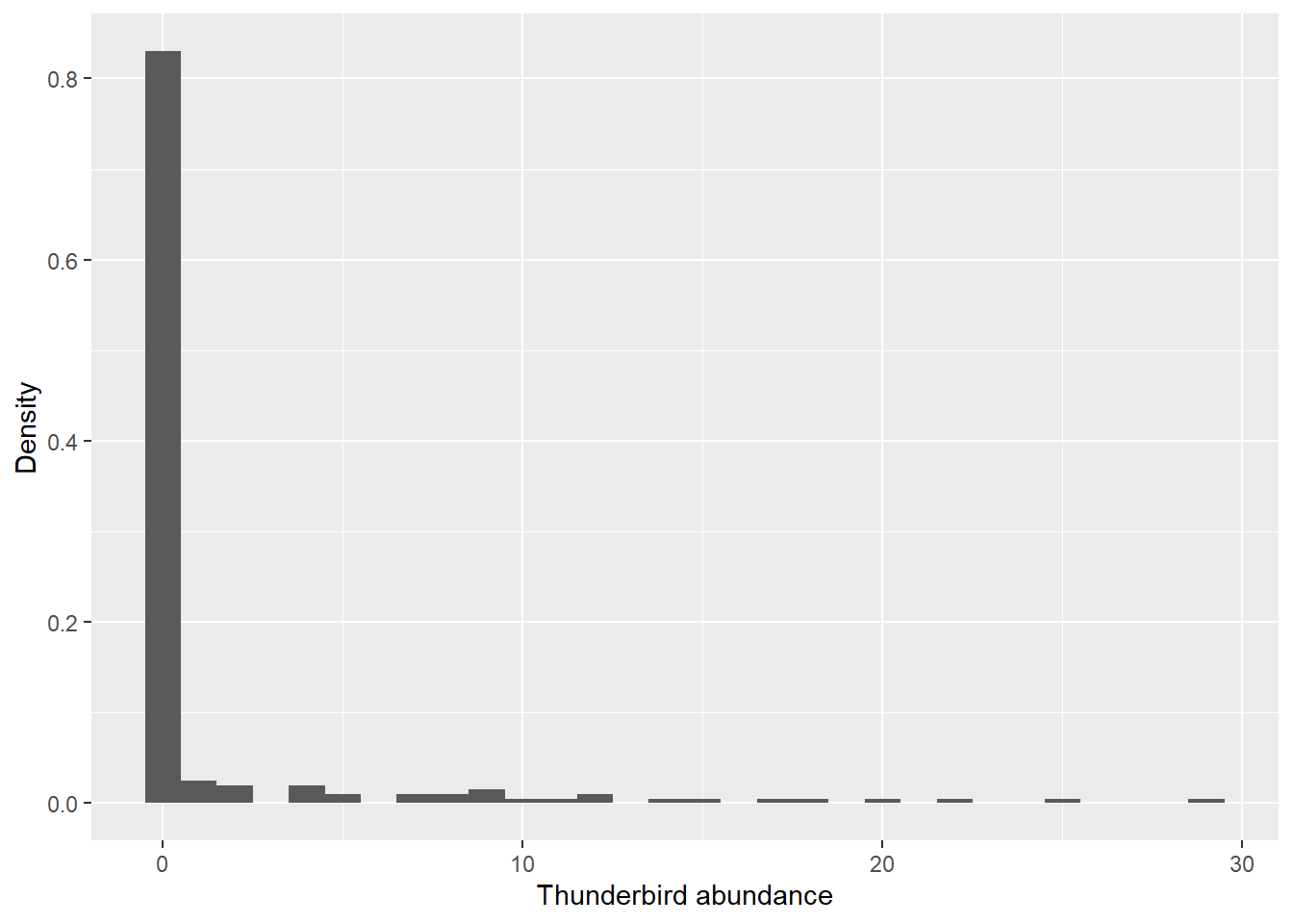
As you can see, we indeed have a really high apparent number of 0s. Our dataset is actually composed of 83% of zeros!!! Zero-inflated indeed.
6.2 Zero-inflated Poisson (ZIP)
Before calling for reinforcements, why don’t we start with something familiar. Just to get us an idea of what we are dealing with. Let’s begin with a simple Poisson regression:
poisson.mod <- glm(y ~ storm + horned.serpents,data=thunderbird.data,family="poisson")Now, using the check_zeroinflation function from the performance package, we can check for zero-inflation:
check_zeroinflation(poisson.mod)# Check for zero-inflation
Observed zeros: 166
Predicted zeros: 75
Ratio: 0.45Model is underfitting zeros (probable zero-inflation).Indeed…
We’re not going to be able to escape it. We’re going to have to tackle this zero-inflation. The zeroinfl function in the pscl package uses a similar structure as the glm and glm.nb functions. We define our model, enter the data, and specify the distribution we want to consider.
ZIP.mod <- zeroinfl(y ~ storm + horned.serpents, data = thunderbird.data, dist="poisson")
summary(ZIP.mod)
Call:
zeroinfl(formula = y ~ storm + horned.serpents, data = thunderbird.data,
    dist = "poisson")

Pearson residuals:
    Min      1Q  Median      3Q     Max
-0.7552 -0.4561 -0.3542 -0.2822  8.7287

Count model coefficients (poisson with log link):
                Estimate Std. Error z value Pr(>|z|)
(Intercept)      1.99453    0.07194  27.725   <2e-16 ***
storm           -0.09468    0.06061  -1.562    0.118
horned.serpents  0.49369    0.04946   9.981   <2e-16 ***

Zero-inflation model coefficients (binomial with logit link):
                Estimate Std. Error z value Pr(>|z|)
(Intercept)     1.647042   0.201186   8.187 2.69e-16 ***
storm           0.585944   0.215964   2.713  0.00666 **
horned.serpents 0.006127   0.201017   0.030  0.97569
---
Signif. codes:  0 '***' 0.001 '**' 0.01 '*' 0.05 '.' 0.1 ' ' 1

Number of iterations in BFGS optimization: 23
Log-likelihood: -199.4 on 6 Df
An important note: as mentioned earlier, the model is actually a combination of two separate subprocesses: a count data model and a zero-inflation model. zeroinfl allows use to either specify both models at the same time, or separately. If we use a formula of type y ~ x1 + x2, then the same variables are employed in both components. By using | however, we can enter different formulas for each component: first the count model, then the zero-inflation model. For example, the formula y ~ x1 | x2 would describe a case where counts are related to variable x1, while zero-inflation is controlled by variable x2.
6.3 Zero-inflated Negative Binomial (ZINB)
Now, before we try to look into our results in more details, did you catch it? Did you notice we forgot to check for one thing? Yes, that’s right, we should also have checked for overdispersion! Let’s fix that mishap right away:
check_overdispersion(poisson.mod)# Overdispersion test
dispersion ratio = 11.254
Pearson's Chi-Squared = 2216.944
p-value = < 0.001Overdispersion detected.Oops! We do need to account for over-dispersion in our dataset too then! This dataset is a mess, I tell you! Oh well… We just have to modify the distribution used in the zeroinfl() function.
ZINB.mod <- zeroinfl(y ~ storm + horned.serpents, data = thunderbird.data, dist="negbin")
summary(ZINB.mod)
Call:
zeroinfl(formula = y ~ storm + horned.serpents, data = thunderbird.data,
    dist = "negbin")

Pearson residuals:
    Min      1Q  Median      3Q     Max
-0.6279 -0.3957 -0.3161 -0.2499  6.9643

Count model coefficients (negbin with log link):
                Estimate Std. Error z value Pr(>|z|)
(Intercept)      1.98651    0.13246  14.997  < 2e-16 ***
storm           -0.01779    0.12211  -0.146   0.8842
horned.serpents  0.54281    0.11956   4.540 5.62e-06 ***
Log(theta)       1.07509    0.44904   2.394   0.0167 *

Zero-inflation model coefficients (binomial with logit link):
                Estimate Std. Error z value Pr(>|z|)
(Intercept)      1.60581    0.20469   7.845 4.33e-15 ***
storm            0.58884    0.21752   2.707  0.00679 **
horned.serpents  0.04171    0.20684   0.202  0.84021
---
Signif. codes:  0 '***' 0.001 '**' 0.01 '*' 0.05 '.' 0.1 ' ' 1

Theta = 2.9303
Number of iterations in BFGS optimization: 27
Log-likelihood:  -185 on 7 Df
Based on those results and on the input of our resident expert on thunderbirds (Lady Penelope) who just came back from the field, we decide to refine our model. Lady Penelope reminded us that thunderbirds are hypothesized to avoid stormy areas, but in calmer areas are expected to flourish as their food source (the horned serpents) increases. Therefore, we are going to link horned.serpents to our count model, and only consider storm for the zero-inflation model, by specifying our formula as follows y ~ horned.serpents | storm.
ZINB.mod.2 <- zeroinfl(y ~ horned.serpents | storm , data = thunderbird.data, dist="negbin")
summary(ZINB.mod.2)
Call:
zeroinfl(formula = y ~ horned.serpents | storm, data = thunderbird.data,
    dist = "negbin")

Pearson residuals:
    Min      1Q  Median      3Q     Max
-0.6244 -0.3971 -0.3132 -0.2506  6.8548

Count model coefficients (negbin with log link):
                Estimate Std. Error z value Pr(>|z|)
(Intercept)       1.9947     0.1244  16.028  < 2e-16 ***
horned.serpents   0.5443     0.1163   4.682 2.85e-06 ***
Log(theta)        1.0738     0.4417   2.431   0.0151 *

Zero-inflation model coefficients (binomial with logit link):
            Estimate Std. Error z value Pr(>|z|)
(Intercept)   1.6067     0.2044   7.859 3.86e-15 ***
storm         0.5895     0.2174   2.712  0.00669 **
---
Signif. codes:  0 '***' 0.001 '**' 0.01 '*' 0.05 '.' 0.1 ' ' 1

Theta = 2.9264
Number of iterations in BFGS optimization: 23
Log-likelihood:  -185 on 5 Df
We can now confirm that indeed, our counts increase with the density of horned serpents. When it comes to interpreting the Zero-inflation model coefficients, keep in mind that we are focusing on predicting the proportion of 0s. In this context, a positive coefficient indicates that the proportion of zeros will increase with an increase in the explanatory variable. Here, the higher the storm index, the less likely the thunderbird is to be present.
6.3.1 Goodness of Fit: Likelihood Ratio Test
For good measure, we can see if our model performs better than a null model:
library(lmtest)

lrtest(ZINB.mod.2)
Likelihood ratio test
Model 1: y ~ horned.serpents | storm
Model 2: y ~ 1
#Df LogLik Df Chisq Pr(>Chisq)
1 5 -185.00
2 3 -197.32 -2 24.652 4.434e-06 ***
---
Signif. codes: 0 '***' 0.001 '**' 0.01 '*' 0.05 '.' 0.1 ' ' 1Yeepee! It does! (significant difference, and higher log-likelihood!). We can even compare our ZIP and ZINB attempts:
library(lmtest)

lrtest(ZIP.mod, ZINB.mod)
Likelihood ratio test
Model 1: y ~ storm + horned.serpents
Model 2: y ~ storm + horned.serpents
#Df LogLik Df Chisq Pr(>Chisq)
1 6 -199.43
2 7 -184.97 1 28.927 7.515e-08 ***
---
Signif. codes: 0 '***' 0.001 '**' 0.01 '*' 0.05 '.' 0.1 ' ' 1And tadaaa, the original ZINB significantly improved our fit! As a final check, we can compare our original ZINB model to our refined one:
library(lmtest)

lrtest(ZINB.mod, ZINB.mod.2)
Likelihood ratio test
Model 1: y ~ storm + horned.serpents
Model 2: y ~ horned.serpents | storm
#Df LogLik Df Chisq Pr(>Chisq)
1 7 -184.97
2 5 -185.00 -2 0.0632 0.9689Both models perform equally well, we can save ourselves some covariates, and use the simpler model!
6.4 A note on Hurdle models
The models described above (Zero-Inflated) assume that zeros can emerge from either a zero-inflation process or a count process. Another class of models that can be used for data with excessive zeros are hurdle count models.
Hurdle count models differ from zero-inflated models by completely separating the modeling of the zeros from the counts. There is only one source of zeros: the hurdle component. If the hurdle for modeling the occurrence of zeros is exceeded, then and only then will we use the count model.
In that case, counts are modeled using (typically) truncated Poisson or negative binomial regressions, where the counts have to be \(\geq\) 1.
Hurdle regression models for count data can be fitted in R using the hurdle function from the pscl package, following a similar approach as the one described above for zero-inflated models. Feel free to go down the jackalope hole if you ever wish to by checking its help file: ? pscl::hurdle.