fish.data=data.frame(sitenumber=1:100,
                     fish.population=c(7, 3, 7, 1, 9, 1, 0, 0, 33, 15, 0,
                                       8, 10, 6, 6, 0, 5, 4, 0, 0, 18, 1,
                                       0, 4, 9, 35, 7, 6, 52, 18, 2, 6, 0,
                                       1, 1, 1, 17, 0, 1, 0, 1, 2, 3, 2, 1,
                                       5, 21, 5, 3, 2, 0, 2, 12, 4, 0, 0, 3,
                                       0, 0, 2, 4, 10, 13, 10, 2, 4, 15, 3,
                                       4, 20, 2, 1, 33, 0, 3, 0, 6, 32, 15,
                                       0, 18, 5, 1, 1, 1, 0, 0, 52, 2, 23, 0,
                                       4, 8, 4, 6, 13, 4, 0, 0, 3) ,
                     # Standardized food availability:
                     food=c(0.7726, 0.3052, 0.4091, -0.7749, 0.9618, -0.2377,
                            -1.2015, -0.8639, 1.6418, 1.1006, -1.2936, 0.3786,
                            0.5588, 0.3441, 0.4137, -0.625, 0.5609, -0.2873,
                            -0.7354, -2.353, 1.3576, 0.0096, -1.6573, 0.5267,
                            0.9805, 1.5259, 0.4241, 0.5559, 1.9227, 1.1616,
                            -0.4877, 0.434, -1.3075, -1.2571, -0.4045, 0.3146,
                            1.0496, -1.1584, -0.9643, -0.7425, -0.6268, -0.2768,
                            -0.0564, 0.0732, -0.4332, 0.7553, 1.2763, 0.5868,
                            0.0771, -0.2776, -0.1421, -0.5285, 0.8199, 0.11,
                            -0.4764, -1.189, 0.3835, 0.1221, -0.327, -0.4722,
                            0.4809, 0.9963, 0.8434, 0.9199, -0.2348, 0.308,
                            1.0344, 0.0919, -0.0676, 1.317, -0.2041, -0.4657,
                            1.565, -0.8463, 0.457, -1.1507, 1.0512, 1.7268,
                            1.0127, -0.4697, 1.4311, 0.1237, -0.8073, -0.6794,
                            -0.8374, -0.053, -1.2292, 1.8966, -0.3192, 1.4033,
                            -0.6946, 0.1261, 1.1178, -0.0309, 0.9486, 0.9798,
                            -0.4686, -1.9257, -1.4116, -0.1264)
)4 The Poisson regression
What do you say we expend our horizon, make Ms. Frizzle proud, and open the door to number bigger than one? Let’s take a look at how we could model count data next.
The Poisson regression is the GLM used when the response variable is the result of a -guess what- Poisson distribution1 and the link function is the log function. As previously stated, this is typically where you will start for population counts. The Poisson distribution is brought to us by -you guessed it- the great Siméon Denis Poisson, the same great French mathematician and physicist that also brought you the Poisson’s Equation, the Poisson Integral, and the Poisson Summation Formula. When you get that many things named after yourself, you know you’re cooking! He was pretty much the Simone Biles of his time.
4.1 Data
To see how it functions in practice, let’s take the example of the tarpies’ abundance in Lake Tarpon. We have sampled the fish population in 100 different sites and for each site we recorded the total abundance and the amount of food available. We hypothesize that fish abundance is related to food availability. Here are the data:
A quick look:
plot(fish.population~food,fish.data,xlab="Food",ylab="Tarpies abundance")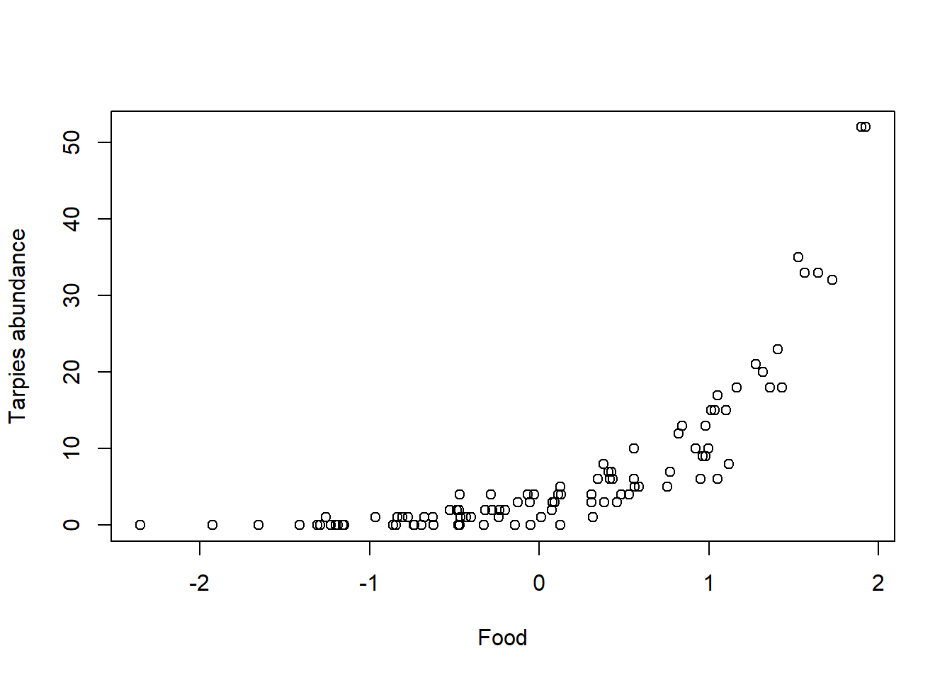
4.2 Estimation
Impatient and just want to jump to doing a Poisson regression? No worries, I got you: you just use the “glm()” function and set the argument “family” to “poisson” (go figure…):
fish.res=glm(fish.population~food, family=poisson, data=fish.data)To analyze the results, as usual, we can get a summary of our model’s results via the well-named function “summary()”.
summary(fish.res)
Call:
glm(formula = fish.population ~ food, family = poisson, data = fish.data)

Coefficients:
            Estimate Std. Error z value Pr(>|z|)
(Intercept)  0.87677    0.07580   11.57   <2e-16 ***
food         1.59823    0.05891   27.13   <2e-16 ***
---
Signif. codes:  0 '***' 0.001 '**' 0.01 '*' 0.05 '.' 0.1 ' ' 1

(Dispersion parameter for poisson family taken to be 1)

    Null deviance: 1090.685  on 99  degrees of freedom
Residual deviance:   92.837  on 98  degrees of freedom
AIC: 365.86

Number of Fisher Scoring iterations: 5
4.3 Diagnostics and Model performance
Before looking at the result though, we need to run a couple of checks…
4.3.1 Checking for overdispersion
An essential assumption underlying the Poisson distribution is that the mean and variance should be equal. If this is not the case, a different approach should be considered.
We can get a quick and rough idea of whether or not overdispersion is an issue for our model by calculating the Dispersion Ratio (i.e., the ratio of the residual deviance over the degrees of freedom) using information from the model summary:
fish.res$deviance/fish.res$df.residual # deviance can also be extracted with deviance(fish.res)[1] 0.9473164If this ratio is close to one (say between 0.9 and 1.1), overdispersion should not be a problem. However, if it is significantly greater than 1, you are likely to be facing overdispersion and will need to call in the big guns to handle that situation.
You can compute an overdispersion test using the check_overdispersion() function from the performance package. This package is a gold mine to look at model performances, in case you had not figured that out yet.
library(performance)
check_overdispersion(fish.res)
# Overdispersion test
dispersion ratio = 0.810
Pearson's Chi-Squared = 79.399
p-value = 0.915No overdispersion detected.It looks like here, we are good to go to use a Poisson distribution to model our tarpies data. Good.
4.3.2 A simple measure of fit
Next, we will want to take a look at the model fit. We can follow a similar approach to what we’ve already done for the logistic regression.
The null deviance and the corresponding degrees of freedom indicate a highly significant difference between fitted values and observed values:
1-pchisq(fish.res$null.deviance,fish.res$df.null) [1] 0(Noticed how I directly extracted the “null.deviance” and the number of degrees of freedom “df.null” from the GLM output?)
Once the predictor is added though, it’s a different story!
1-pchisq(fish.res$deviance,fish.res$df.residual) [1] 0.6283983Now, the fitted values are not significantly different from the observed values. We therefore cannot reject the null hypothesis (i.e., our model prediction and our observed data are similar).
4.3.3 Goodness of Fit: Likelihood Ratio Test
Another way to look at it is to perform a likelihood ratio test, and test directly if our model performs better than a Null model.
We can use the same tools as presented for the logistic regression, either using base R:
anova(fish.res)Analysis of Deviance Table
Model: poisson, link: log
Response: fish.population
Terms added sequentially (first to last)
Df Deviance Resid. Df Resid. Dev Pr(>Chi)
NULL 99 1090.68
food 1 997.85 98 92.84 < 2.2e-16 ***
---
Signif. codes: 0 '***' 0.001 '**' 0.01 '*' 0.05 '.' 0.1 ' ' 1or a dedicated package:
library(lmtest)
lrtest(fish.res)
Likelihood ratio test
Model 1: fish.population ~ food
Model 2: fish.population ~ 1
#Df LogLik Df Chisq Pr(>Chisq)
1 2 -180.93
2 1 -679.85 -1 997.85 < 2.2e-16 ***
---
Signif. codes: 0 '***' 0.001 '**' 0.01 '*' 0.05 '.' 0.1 ' ' 1Here, we can confirm once again that adding our food covariate leads to a significant improvement in the fit of our model to our data. Nothing fishy here!
4.3.4 A look a the residuals
Let’s make sure our residuals are distributed as expected by simulating randomized quantile residuals.
library(performance)
library(qqplotr)

simulated_residuals <- simulate_residuals(fish.res)

plot(simulated_residuals)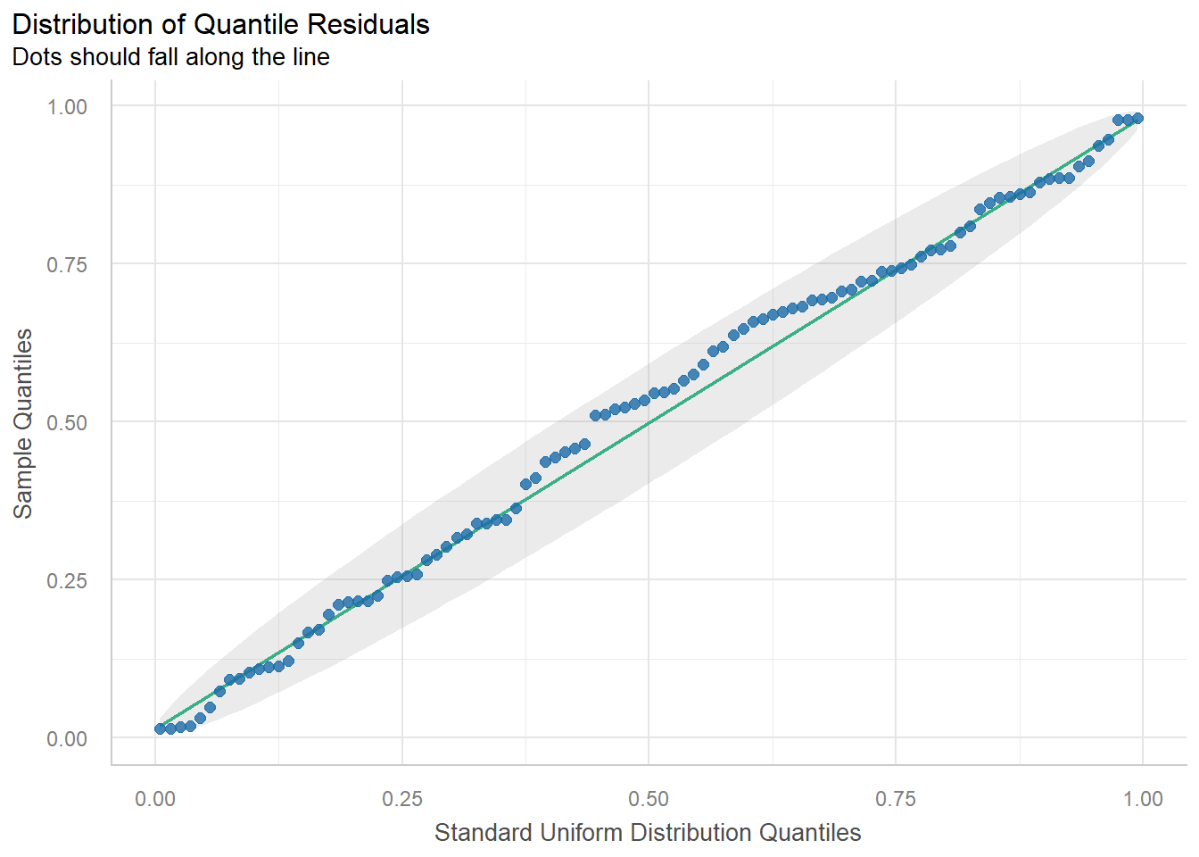
check_residuals(simulated_residuals) OK: Simulated residuals appear as uniformly distributed (p = 0.705).Nothing to see here, we can confidently jump to what we’re all here for. Inferences!
4.4 Inferences
4.4.1 A Closer look
summary(fish.res)
Call:
glm(formula = fish.population ~ food, family = poisson, data = fish.data)

Coefficients:
            Estimate Std. Error z value Pr(>|z|)
(Intercept)  0.87677    0.07580   11.57   <2e-16 ***
food         1.59823    0.05891   27.13   <2e-16 ***
---
Signif. codes:  0 '***' 0.001 '**' 0.01 '*' 0.05 '.' 0.1 ' ' 1

(Dispersion parameter for poisson family taken to be 1)

    Null deviance: 1090.685  on 99  degrees of freedom
Residual deviance:   92.837  on 98  degrees of freedom
AIC: 365.86

Number of Fisher Scoring iterations: 5
Looking at the summary of our model output, we see that we have statistically significant intercept and food effect. We can directly extract the corresponding coefficients from the GLM output:
fish.res$coefficients # or we can get the same information with 'coef(fish.res)'(Intercept) food
0.8767657 1.5982324 We can extract from the specific coefficient value on the log-scale for our food effect.
fish.res$coefficients[["food"]][1] 1.598232Which in turn can be used to express our population growth rate depending on the food availability. Since this coefficient is on the log scale, we need to use the inverse function of the log, i.e. the exponential, in order to get this information.
exp(fish.res$coefficients[["food"]]) [1] 4.944285Every time we add one food unit on the standardized scale, the tarpies population will get 4.9 times larger. In a real life situation, we would also back transform the standardized “food” covariate to give a clearer ecological description of our dynamic.
4.4.2 Plotting the fit
As for the previous fitted models, we can plot the fitted line, but this time, let’s ‘prettify’ it with ggplot2 for good measure:
food.new <- seq(min(fish.data$food), max(fish.data$food), length.out = 100) # Creating new values of the covariates for which we want to predict the response variable
resp.pred=data.frame(food=food.new)

resp.pred$pred <- predict(fish.res, newdata=resp.pred, type="response") # Predictions


library(ggplot2)

gg.poisson <- ggplot() +
  geom_point(aes(x=food,y=fish.population), data=fish.data) +
  geom_line(aes(x= food,y=pred ),col="red",data=resp.pred) + # Fitted values
  labs( title="Fish abundance depending on food resources",
        x="Food",
        y=" Abundance")+
  theme_minimal()
 gg.poisson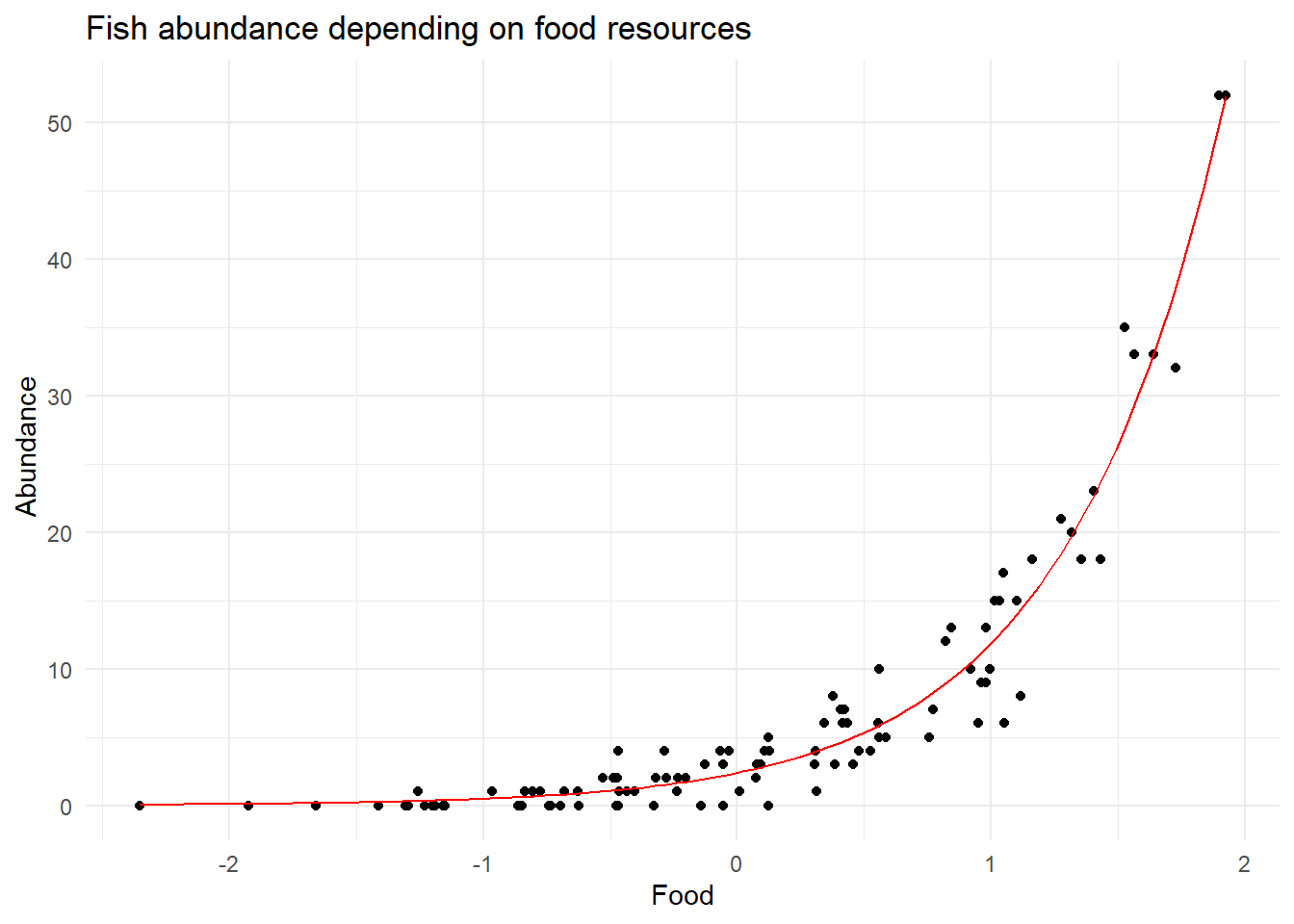
And compute and plot the prediction’s 95% confidence interval:
pred.linkscale <- predict(fish.res, newdata=resp.pred, se=T)
pred.linkscale.CI2.5  = pred.linkscale$fit-1.96*pred.linkscale$se.fit
pred.linkscale.CI97.5 = pred.linkscale$fit+1.96*pred.linkscale$se.fit

resp.pred$CI2.5  = family(fish.res)$linkinv(pred.linkscale.CI2.5)
resp.pred$CI97.5 = family(fish.res)$linkinv(pred.linkscale.CI97.5)


gg.poisson.2 <- gg.poisson +
  geom_ribbon(aes(x=food, ymin = CI2.5,ymax = CI97.5),
              alpha=0.15,data=resp.pred)
gg.poisson.2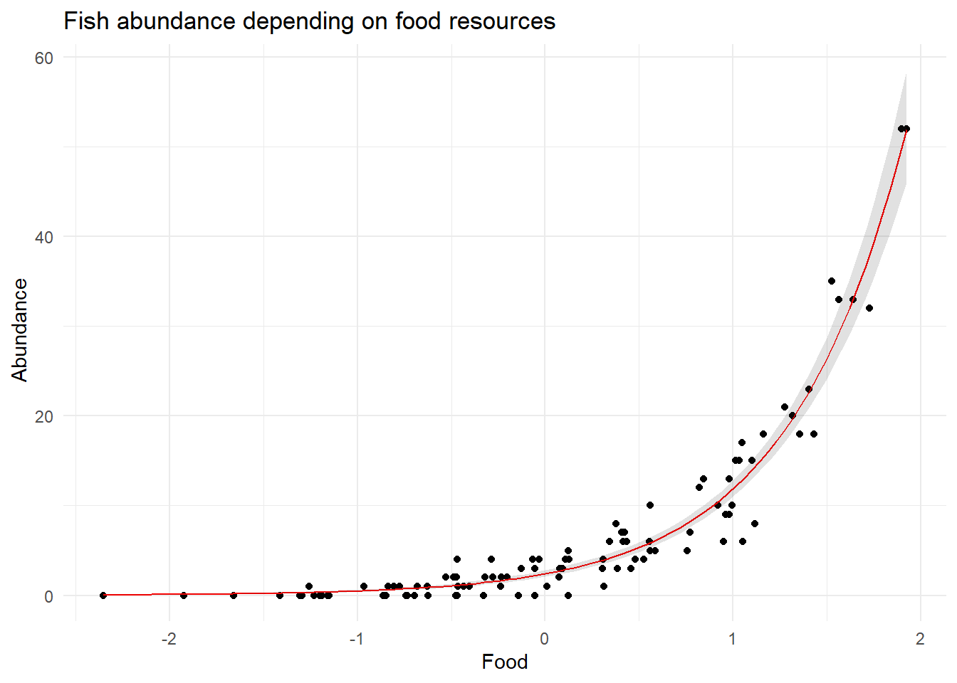
I know… Beautiful, right?